Algotrading: Can a Simple Bollinger Bands Strategy Beat Buy & Hold?

The Dream: Automatic Profits While You Sleep

If you’ve ever watched a stock chart dance up and down and thought:

"What if my computer could trade for me while I’m at work?"

…welcome to the world of algorithmic trading (a.k.a. algotrading).

In short, algotrading is about turning your trading ideas into code that automatically buys and sells based on clear rules – no emotions, no panic, no coffee-fueled late-night "hunches".

It sounds incredible. You feed in some data, apply a formula, and voilà – passive income, right?

Well… almost.
Let’s build a real example and see how close we can get.

Our Plan

We will:

1. Take a simple trading idea: using Bollinger Bands.
2. Write it as a strategy using Backtrader.
3. Compare its performance to a "boring" buy & hold.
4. Add trading costs (commissions).
5. See who wins – the robot or the patient investor.

Our "arena" will be the S&P 500 ETF (SPY) between 2015-2025.

What Are Bollinger Bands?

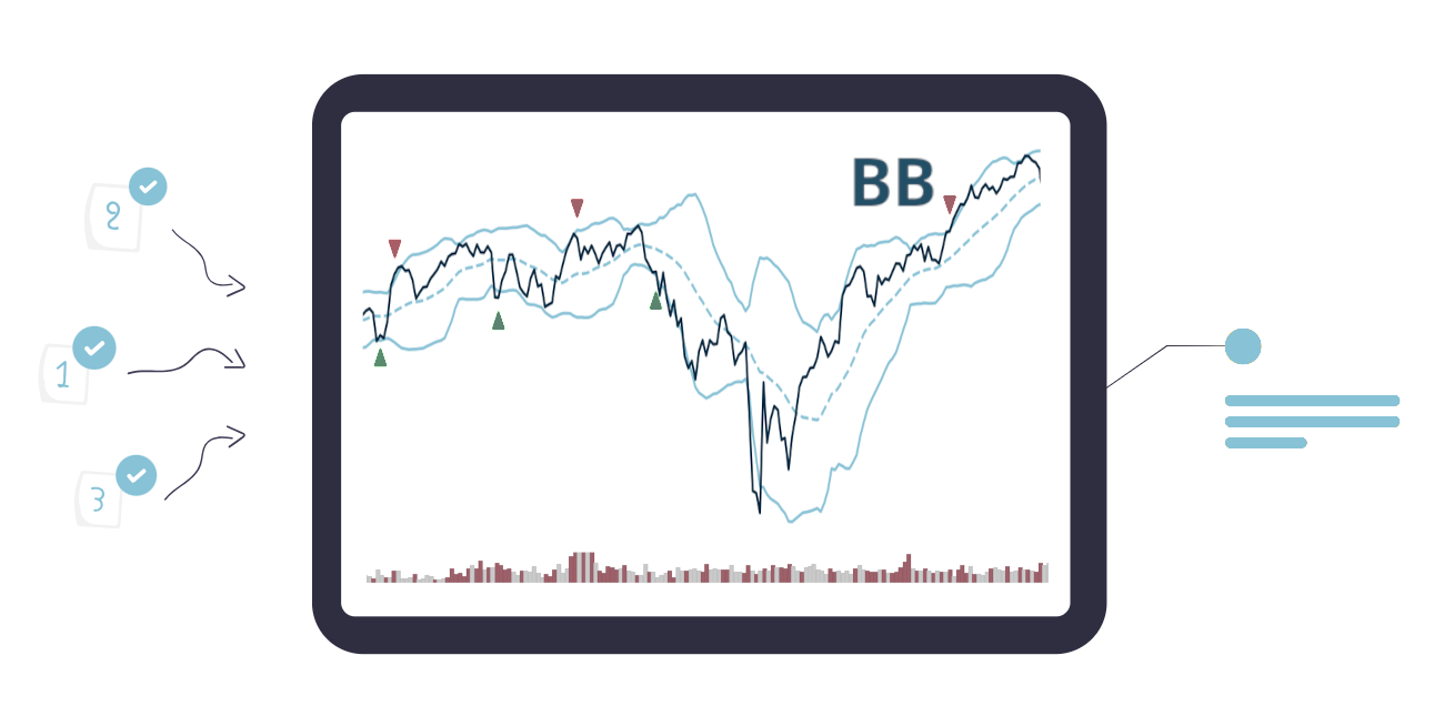
Bollinger Bands are a classic tool invented by John Bollinger in the 1980s.
They’re like elastic boundaries around the price – expanding when volatility grows, contracting when it calms down.

They consist of:

• Middle Band: a moving average (usually 20 days).
• Upper Band: the average + 2 standard deviations.
• Lower Band: the average − 2 standard deviations.

When the price:

• drops below the lower band = it might be "too cheap": buy
• rises above the upper band = it might be "too expensive": sell

It’s like a rubber band around price. When stretched too far, it "snaps back" – at least, that’s the theory.

Setting Up Our Environment

Let’s install the tools first.

pip install backtrader yfinance pandas matplotlib

We’ll use a few popular Python libraries to bring our strategy to life. Backtrader will serve as the backtesting engine – it runs our trading logic, executes virtual trades, and tracks performance. Yfinance will download free historical market data directly from Yahoo Finance, so we can easily test strategies on real-world price movements. Pandas handles all the data manipulation, making it simple to clean and organize our datasets. Finally, matplotlib will take care of the plotting, helping us visualize price charts, indicators, and trading signals in a clear, intuitive way.

The Bollinger Band Strategy Code

Now let’s code it.

We’ll fetch 10 years of `SPY` data, create a Bollinger Bands based strategy, and test it against a "buy & hold" baseline.

import backtrader as bt
import yfinance as yf
import pandas as pd


def download_data():
    df = yf.download("SPY", start="2015-10-01", end="2025-10-01", group_by=None)

    if isinstance(df.columns, pd.MultiIndex):
        df.columns = df.columns.get_level_values(-1)

    df = df[["Open", "High", "Low", "Close", "Volume"]]
    df.index = pd.to_datetime(df.index)
    return df


class BollingerBandsStrategy(bt.Strategy):
    """
    risk_per_trade: float between 0 and 1
    Specifies the fraction of available cash allowed to be used per trade.
    """

    params = dict(period=20, devfactor=2, risk_per_trade=1.0)

    def __init__(self):
        super().__init__()
        self.bb = bt.ind.BollingerBands(
            period=self.p.period, devfactor=self.p.devfactor
        )

    def next(self):
        if not self.position:
            if self.data.close[0] < self.bb.lines.bot[0]:
                self.buy(size=self.calculate_position_size())

        else:

            if self.data.close[0] > self.bb.lines.top[0]:
                self.sell(size=self.position.size)

    def calculate_position_size(self):
        available_cash = self.broker.getcash()
        available_cash *= self.p.risk_per_trade
        return int(available_cash / self.data.close[0])


def run_strategy(strategy_name, strategy, data, cash):
    cerebro = bt.Cerebro(stdstats=False)

    cerebro.addobserver(bt.observers.Value)
    cerebro.addobserver(bt.observers.Cash)
    cerebro.addobserver(bt.observers.Trades)
    cerebro.addobserver(bt.observers.DrawDown)
    cerebro.addobserver(bt.observers.BuySell)

    cerebro.addanalyzer(bt.analyzers.SharpeRatio, _name="sharpe")
    cerebro.addanalyzer(bt.analyzers.DrawDown, _name="drawdown")

    cerebro.adddata(data)
    cerebro.addstrategy(strategy)
    cerebro.broker.setcash(cash)

    results = cerebro.run()

    result = results[0]
    analysers = result.analyzers
    sharpe = analysers.sharpe.get_analysis()
    drawdown = analysers.drawdown.get_analysis()

    print(f"Strategy: {strategy_name}")
    print(f"Final value: {cerebro.broker.getvalue():.2f}")
    print(f"Sharpe ratio: {sharpe['sharperatio']:.2f}")
    print(f"Max drawdown: {drawdown['max'].moneydown:.2f} ({drawdown['max'].drawdown:.2f}%)")

    cerebro.plot(iplot=False)


if __name__ == "__main__":
    df = download_data()
    data = bt.feeds.PandasData(dataname=df)
    cash = 10000
    run_strategy("Bollinger Bands", BollingerBandsStrategy, data, cash)

The Results

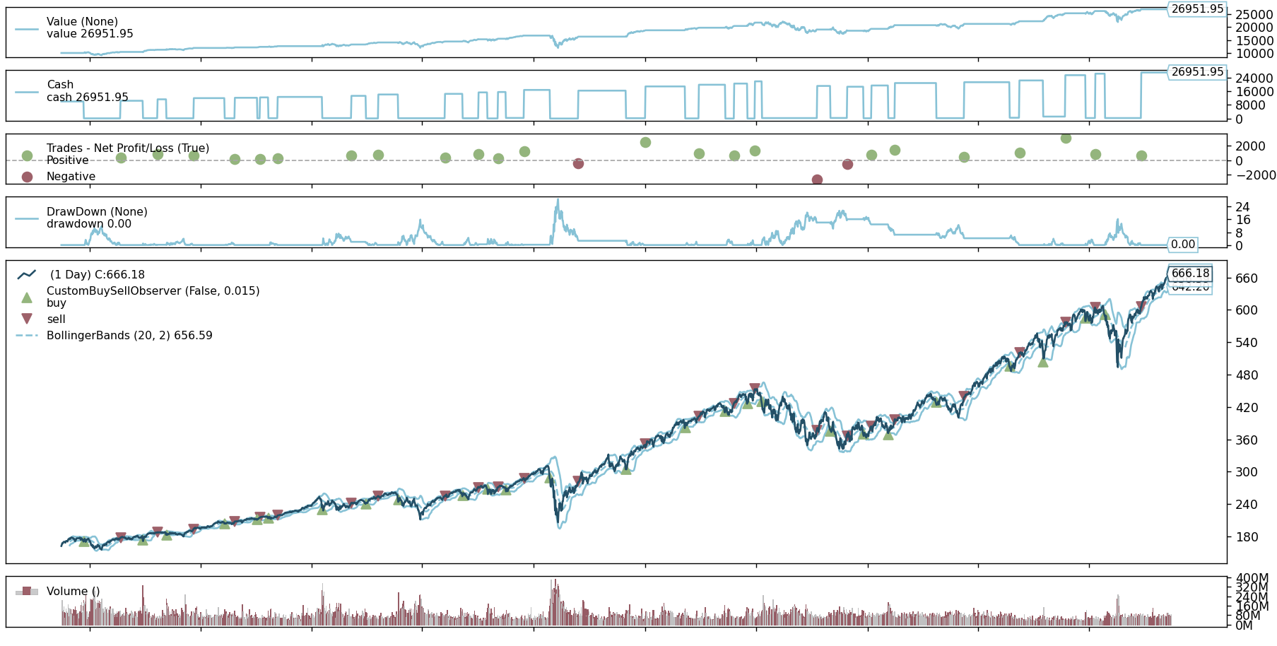
When you run the code, Backtrader will print something like:

Final value: 26951.97
Sharpe ratio: 0.79
Max drawdown: 4825.56 (28.75%)

In addition, you’ll see a chart with price, bands, and buy/sell points:

After zooming:

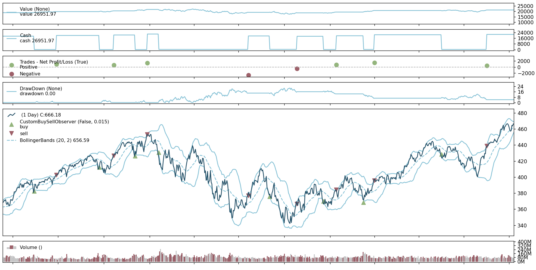
Note: probably your chart looks slightly different as I have custom styling applied. In a separate article I will show you how can you style your backtrader graph.

At first, it looks impressive – your strategy does make money – WOOOHOOOO! You started with 10000 and now you have 26951, which is a 169% return. However, let's compare these results with the benchmark to see how good they really are.

Benchmark

We can create a straightforward buy-and-hold strategy in backtrader which we will use as our benchmark.

# ...

class BuyAndHold(bt.Strategy):
    def __init__(self):
        self.has_bought = False

    def next(self):
        if not self.has_bought:
            max_position_size = int(self.broker.getcash() / self.data.close[0])
            if max_position_size > 0:
                self.buy(size=max_position_size)
                self.has_bought = True
                
                
def run_benchmark_strategy(data, cash):
    cerebro = bt.Cerebro()
    cerebro.adddata(data)
    cerebro.addstrategy(BuyAndHold)
    cerebro.broker.setcash(cash)
    cerebro.addanalyzer(bt.analyzers.SharpeRatio, _name="sharpe")
    cerebro.addanalyzer(bt.analyzers.DrawDown, _name="drawdown")
    cerebro.addanalyzer(bt.analyzers.AnnualReturn, _name="annualreturn")

    results = cerebro.run()

    analysers = results[0].analyzers
    sharpe = analysers.sharpe.get_analysis()
    drawdown = analysers.drawdown.get_analysis()
    annualreturn = analysers.annualreturn.get_analysis()

    print(f"\nBenchmark: Buy & Hold")
    print(f"Final value: {cerebro.broker.getvalue():.2f}")
    print(f"Sharpe ratio: {sharpe['sharperatio']:.2f}")
    print(f"Max drawdown: {drawdown['max'].moneydown:.2f} ({drawdown['max'].drawdown:.2f}%)")
    print(f"Annual returns:")
    for year in annualreturn:
        print(f"{year}: {annualreturn[year]*100:.2f}%")

if __name__ == "__main__":
    df = download_data()
    data = bt.feeds.PandasData(dataname=df)
    cash = 10000
    run_benchmark_strategy(data, cash)

Our results look like this:

Benchmark: Buy & Hold
Final value: 40855.13
Sharpe ratio: 0.96
Max drawdown: 6951.43 (33.33%)
Annual returns:
2015: 7.89%
2016: 11.76%
2017: 21.31%
2018: -4.50%
2019: 30.74%
2020: 18.11%
2021: 28.44%
2022: -18.03%
2023: 25.92%
2024: 24.70%
2025: 14.57%

So, in this case you would have started with 10000$ and after 10 years you would have 40855$, which is a 308% return! Surprisingly, doing nothing – just buying and holding – beats your active strategy heavily.

Why? Because:

• The strategy often sits in cash while SPY keeps climbing.
• Markets trend more than they mean-revert in long bull runs.

In sideways or choppy years, Bollinger Bands might shine.
But over a decade of rising prices, buy & hold tends to win by a mile.

The Cost of Being Clever

Adding commissions can also make things worse. Backtrader allows you to simulate transaction fees. For example, to reflect tiered commissions for shares in the US using Interactive Brokers, you could use the following snippet:

import backtrader as bt


class UsTieredIbCommissionScheme(bt.CommInfoBase):
    params = dict(
        commission=0.0035,           # $0.0035 per share
        min_commission=0.35,         # minimum per order
        max_commission_rate=0.01,    # maximum fraction of trade value
        leverage=1.0,
        stocklike=True,
        commtype=bt.CommInfoBase.COMM_FIXED,
    )

    def _getcommission(self, size, price, pseudoexec):
        comm = abs(size) * self.p.commission
        trade_value = abs(size) * price 
        max_commission = trade_value * self.p.max_commission_rate
        return min(max(comm, self.p.min_commission), max_commission)
    
# ...

cerebro.broker.addcommissioninfo(UsTieredIbCommissionScheme())

You could also update your code to be able to count transactions and calculate the total comissions paid:

import backtrader as bt


class CommissionAwareStrategy(bt.Strategy):
    def __init__(self):
        self.total_commission = 0
        self.transaction_count = 0

    def notify_order(self, order):
        if order.status in [order.Completed]:
            if order.isbuy():
                self.transaction_count += 1
            elif order.issell():
                self.transaction_count += 1

    def notify_trade(self, trade):
        if trade.isclosed:
            self.total_commission += trade.commission


# Make BollingerBandsStrategy extend CommissionAwareStrategy
class BollingerBandsStrategy(CommissionAwareStrategy):
# ...

# Print results
results = cerebro.run()
result = results[0]
print(f"Total number of transactions: {result.transaction_count}")
print(f"Total commissions paid: ${result.total_commission:.2f}")

In this case the Bollinger Bands based algorithm executed 56 transactions and the total comissions paid was 19.60$. Unfortunately, in Europe – depending on the specific country – commissions are usually much higher.

It’s the perfect real-world reminder:

Trading less often is sometimes the best strategy.

Even professional quant funds obsess over execution cost, slippage, and spreads – because these tiny percentages add up fast.

Step 6: Lessons Learned

So what did we discover?

1. You can build a working trading algorithm in under 100 lines of Python.
   It’s fun, educational, and feels powerful.
2. Simple ideas aren’t enough.
   What looks great in theory can lose to a basic buy & hold portfolio.
3. Markets have regimes.
   Mean-reversion works best in sideways markets; trend-following works best in long trends.
4. Backtesting ≠ real profits.
   The future never behaves like the past – and slippage, taxes, and emotions all matter.

What’s Next?

Ideas for future posts to explore this topic in more depth:

• Optimize Bollinger parameters.
• Improve risk management and position sizing.
• Compare different indicators like RSI or MACD.
• Try machine learning models.

But before we go there – take a moment to appreciate the quiet wisdom of buy & hold.
Sometimes the simplest algorithm is the one that does nothing at all.

Final Thoughts

Algorithmic trading is like chess against the market.
You can teach your computer the rules – but the market always plays black, and it’s faster, richer, and less emotional than you are.

Still, coding strategies like this is incredibly rewarding.
You learn data analysis, finance, and probability – and you can test ideas without losing real money.